❝....the fact that it takes four whole chapters to cover the process of extracting a reasonable signal from a record groove indicates to me that there is something amiss with the whole concept.❞... Small Signal Audio Design by Doug Self 8
The signal recorded onto a vinyl record is pre-equalised, whereby the bass is cut and the treble boosted during the cutting of the master disc. If this isn’t done, the big “wiggles” of the musical bass frequencies tend to throw the needle out of the groove on playback, or break through to an earlier rotation of the spiral groove in cutting.
Additionally, by boosting the treble, a better overall noise performance is secured. Replay electronics is therefore required to present a complimentary characteristic. At the start of the LP-era, various equalisation characteristics were defined. However the characteristic defined by the Recording Industries Association of America is now universally adopted, and the replay circuit is always dubbed the RIAA preamplifier.
The hardware circuit must combine this equalisation function with gain, to raise the small signals from the phono cartridge (see right panel) to a level suitable to switching and control in the preamplifier or mixer. The issues in combining these features are labyrinthine — hence Doug Self's comment.
We look at the history of RIAA preamp's on this page, we explore their various shortcomings and why many of the functions are better performed in software as in Stereo Lab.
The equalisation
The transfer function of the pre-equalisation applied to the disc-cutter is given by the transfer function,
where T1 = 3180µS, T2 = 318µS and T3 = 75µS. A circuit which gives a close approximation to this characteristic is given on the page looking at the pre-emphasis equalisers used in Neumann lathes
The complementary, replay characteristic is the inverse of the pre-equalisation transfer function given above. That’s to say,
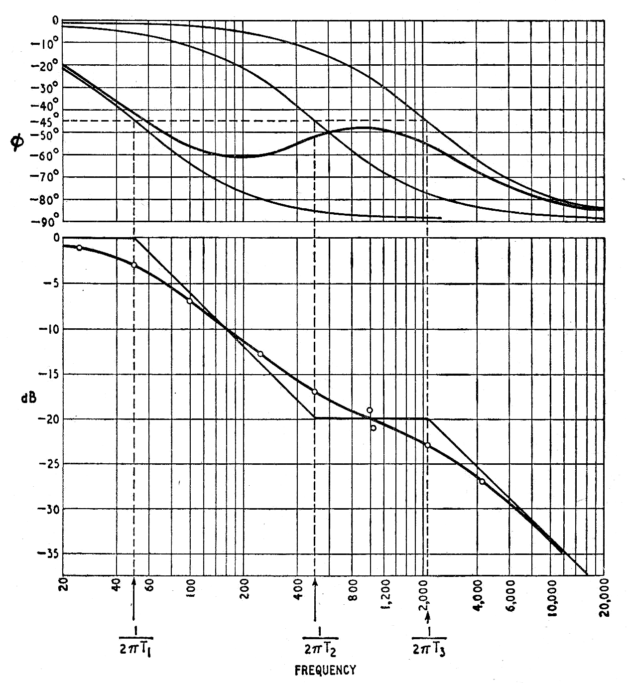
The gain and phase plot of the replay transfer-function (B) are plotted in the figure below for reference.
RIAA replay characteristic indicating amplitude and phase response of the transfer function given in equation B
Provided the time-constants are the same on the replay side, if we multiply this second equation by the first, all the terms cancel out leaving unity; meaning that the overall encode-decode process is transparent and the reproduced music will retain its original frequency response.
Knowing that the combined effect of multiple filter networks has its mathematical equivalent in the multiplication of individual transfer functions, means we can infer that the correct, combined transfer-function may be synthesised from the combination of two, simple networks with the form,
H(jω) = 1/(1 + jωT)
And a third network of the form,
H(jω) = (1 + jωT).
Here we hit a slight, practical complication. Although, in principle, it would be possible to combine the circuits with simple transfer functions together, in practice the impedances of the various networks interfere with each other unless they are separated by buffer amplifiers to isolate one from the other. Such an approach is certainly feasible, but it would be complicated and would probably add to the electrical noise generated.
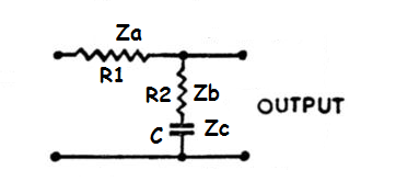
Fortunately, there are simple circuits which may be designed to do double-duty. Such a circuit is given here. It is known as a step-circuit or a shelving-equaliser. This type of circuit is very widely used in analogue audio.
This circuit is in the form of a potential divider, with the slight complication that here, the lower limb is formed by the series connection of a resistor and capacitor. Applying Ohm’s law, we can say that Vout will be related to Vin by the following relationship,
Vout / Vin = Zb + Zc / (Za + Zb + Zc)
Substituting the impedance values for Za, Zb and Zc, we get,
Vout/ Vin = [(1/jωC) + R2] / [R1 + R2 + (1/ jωC)]
If we multiply top and bottom by jωC, we derive,
Vout/ Vin = (1 + jωC.R2) / (jωC (R1 + R2) + 1)
Which we can express as,
H(jω) = (1 + jωT1) / (1 + jωT2)
Where T1 = (R1 + R2)C and T2 = R2.C.
We can see that, with this circuit, we are two-thirds of the way towards the overall RIAA correction transfer function (equation B). All that is required is a further network with the response,
H(jω) = 1 / (1 + jωT3) , and the job is done.
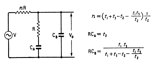
Such an approach could certainly form the basis of a practical equaliser, although usually the shelving equaliser is combined with the final RC low-pass in a combined circuit, the values being cleverly “tweaked” to account for the interaction of the various impedances. Such a circuit is illustrated below along with the design equations.
Practical, passive RIAA replay equalisation circuit. (Note that in these equations, the time constant order is reversed compared with above so that t1 = 75µS, t2 = 318µS and t3 = 3180µS)
It can be demonstrated that the frequency response of the network above is exactly the same as the impedance variation with frequency seen looking back into the output terminals of the network, so that this network may be used directly in the feedback network of an amplifier to get the desired replay characteristic combined with the necessary voltage gain.
Maximum signals from a phono cartridge
Moving magnet (MM) cartridges
Remember that Faraday realised that it took a moving magnet to induce a moving electric-field (a current), so, an electromagnetic pickup is sensitive to the velocity with which the magnet is “wiggled” inside the pickup coils. Pickup sensitivities are therefore specified in terms of the RMS signal voltage due to the velocity of the stylus in the modulated groove; usually given in terms of centimetres per second (cm/s).
Moving-magnet cartridges are more or less standardised in terms of output and load requirement and virtually all models produce around 5mV RMS @ 5cm/s recorded velocity at 1kHz with about 20% variation above and below this figure.
Virtually all of these cartridges are happy with a load of 47k with some capacitance around 200pF.
Velocity limits in recording
The practical velocity limit when cutting a record is 50cm/s peak velocity. Beyond this limit, the cutter will trash the groove it's just made! 50cm/s peak velocity is equivalent to 35cm/s RMS which is 7 times (17dB) above the nominal NAB recording standard level of 5cm/s RMS.
For a nominal MM cartridge output of 5mV @ 5cm/s RMS. This implies that the maximum RMS output cannot ever be greater than 7 times 5mV RMS = 35mV RMS.
Line-up
We have discovered that, if the analogue to digtal converter is aligned so that standard recording level is set -17dBFS, it does show that, when recording a very loud LP record, peaks do indeed reach to 0dBFS. But there isn't any room to spare. So this calibration seems a bit low.
Noel Keywood's article on the Hi-Fi World's website concerning the testing of hardware phono preamplifiers says,
❝MM cartridges a phono stage should ideally be able to accept 40mV input before overload.❞13
This is 40mV/5mV or 8 times above standard level. This is equivalent to standard level being -18dB below full-scale. The extra 1dB (10%) seems worthwhile. This is the final recommendation therefore:
Standard recording level should be set so as to indicate -18dBFS when recording a needle-drop.
For electrical calculations we can assume the maximum input to an MM phono stage to be 113mV pk-pk (40mV RMS).14
Moving-coil (MC) cartridges
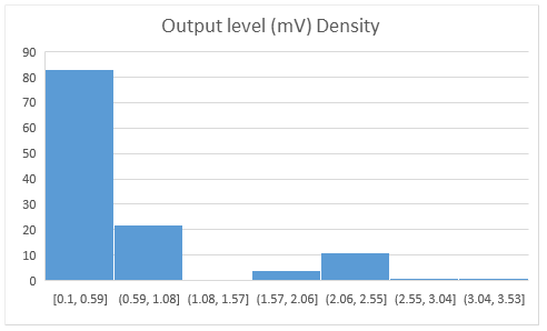
The output voltage level of moving-coil cartridges is much less standardised then it is for moving-magnet types. We surveyed the over 130 models on the market from £200 to £13,500 in spring 2020 and derived the following histogram.
The lion's share of the models are in the 0.2mV to 0.6mV (at 5cm/s velocity). This is still a large range by moving-magnet standards, but a well engineered preamplifier should be able to accomodate a 10dB level-range.
The existence of a relatively new breed of phono cartridge known as the high-output moving-coil is signalled on the graph by the bars in the 1.5mV to 2.5mV range. These are the result of employing large pickup coils and/or stronger magnets. And there exist a significant number of half-way-house models in the 0.5mV to 1mV range.
The overall picture is therefore of transducers with an output range of 24dB, the inevitable result of which is the preamplifier being over- or under-driven depending on the assumptions made by the designer. Many models are too high for the "standard" assumption (of 0.5mV@5cm/s) for a moving-coil amplifier and too low for a standard moving-magnet sensitivity amplifier.
It is entirely possible to equalise for the RIAA pre-emphasis using the passive equaliser developed above. But this is very inconvenient if operated at the signal levels which emanate from practical phono cartridges (see panel), so there is the need to provide voltage gain before the equaliser.
The only disadvantage of this approach is that the electrical signals which are provided by a velocity-sensitive pickups (and and most are) inevitably exaggerate high-frequencies. These signal components contribute to the high crest-factor of the waveforms prior to de-emphasis. So, the amplifier before the equaliser must provide good headroom (or freedom from overload).
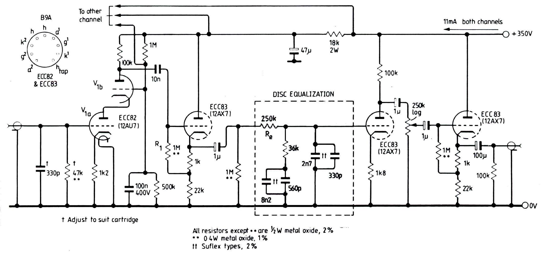
This, in fact, exaggerated requirement (see sidebar and note. 14) has led to some quite exotic design ideas over the years. An example is the circuit given above in which the amplification prior to the passive equaliser is performed by no less than three tubes (valves) on a 300 volt supply: a cascode amplifier stage, for high-gain and low-noise, and a cathode-follower for a low output impedance.4
More conveniently for cost-effective, commercial design, the equalisation is combined with the amplification stage. In this way, the amplifier is never called upon to reproduce the amplified, "raw" signal from the pickup and the headroom requirement may be relaxed.
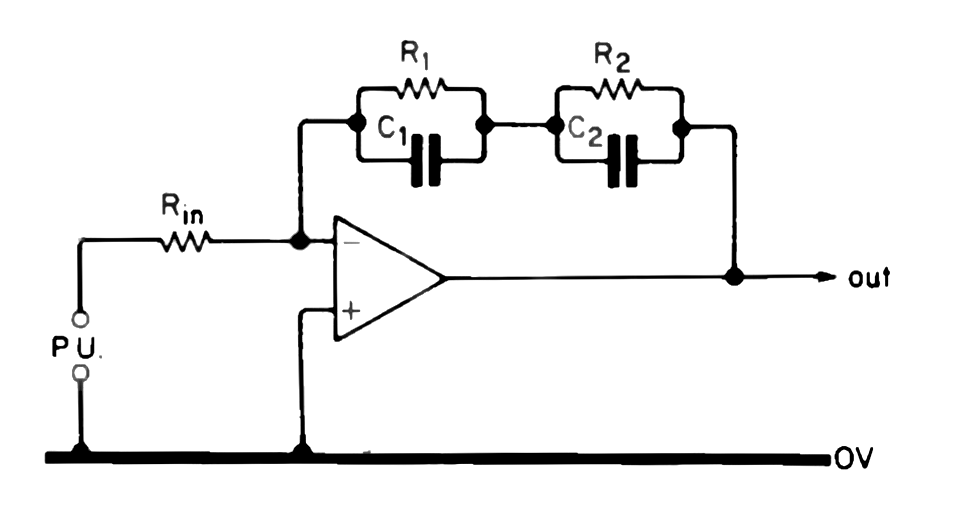
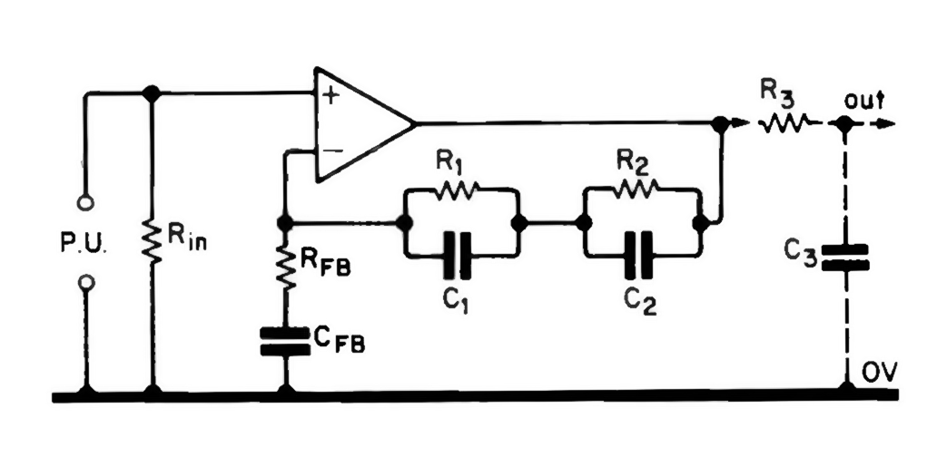
The question then becomes, should the phono cartridge signal to the equalising amplifier be fed to the inverting or non-inverting input? The two possible approaches are illustrated below.
In both circuits, the negative feedback network (which provides the equalisation), connects the output and the inverting input - as expected. But, in the left-hand circuit, the signal feeds the inverting input of the amplifier too (via Rin). Whereas, in the right-hand circuit, the signal feeds the non-inverting input.
The left-hand arrangement is a, so-called, virtual-earth amplifier circuit. The term derives from the observation that, proviving the gain of the amplifier is very large, the inverting input will always be "virtually" at the same potential as the non-inverting (+) input of the summing amplifier which is itself grounded or earthed.
The advantage of this circuit arrangement is that the gain keeps on falling with frequency, all the way to zero — just as the transfer-function (equation B) demands. Whereas, the gain of the right-hand, non-inverting circuit falls to a minimum of one. This - depending on the overall design - may cause problems in the uppermost octaves of the frequency-response. A solution to this shortcoming is to add a further pole in the form of a RC filter after the main circuit as is illustrated with the dotted components.
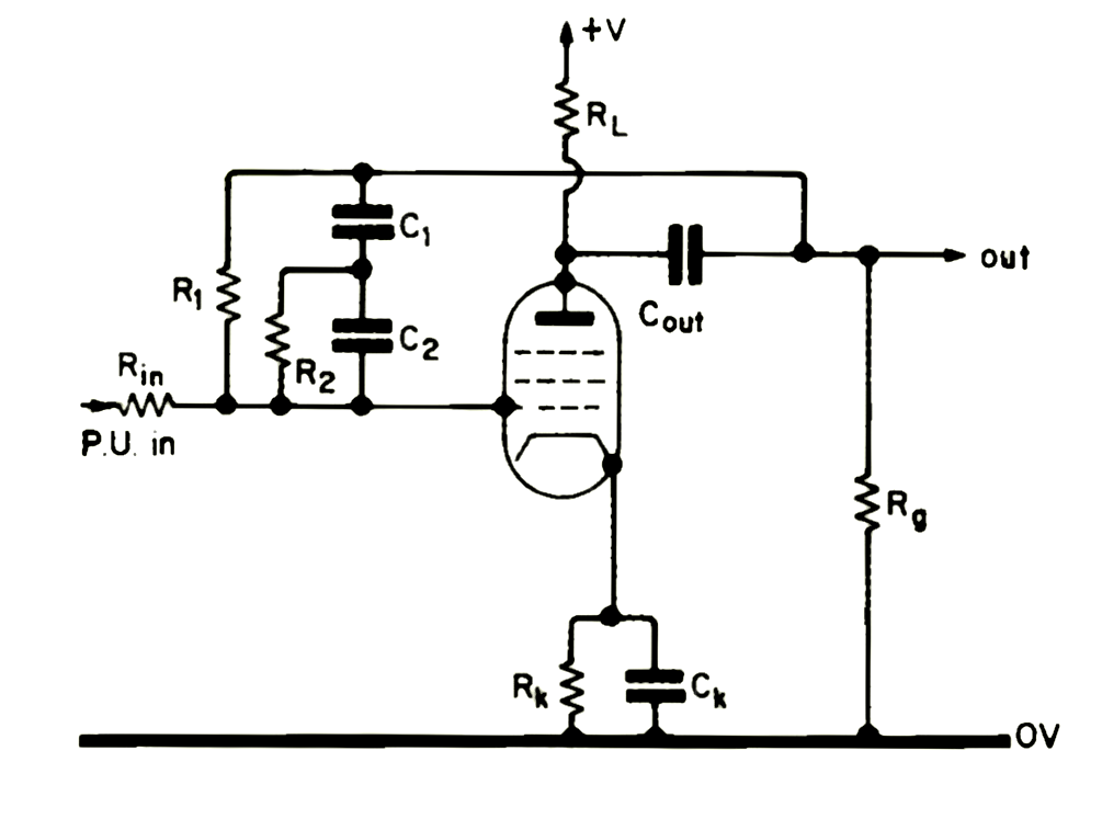
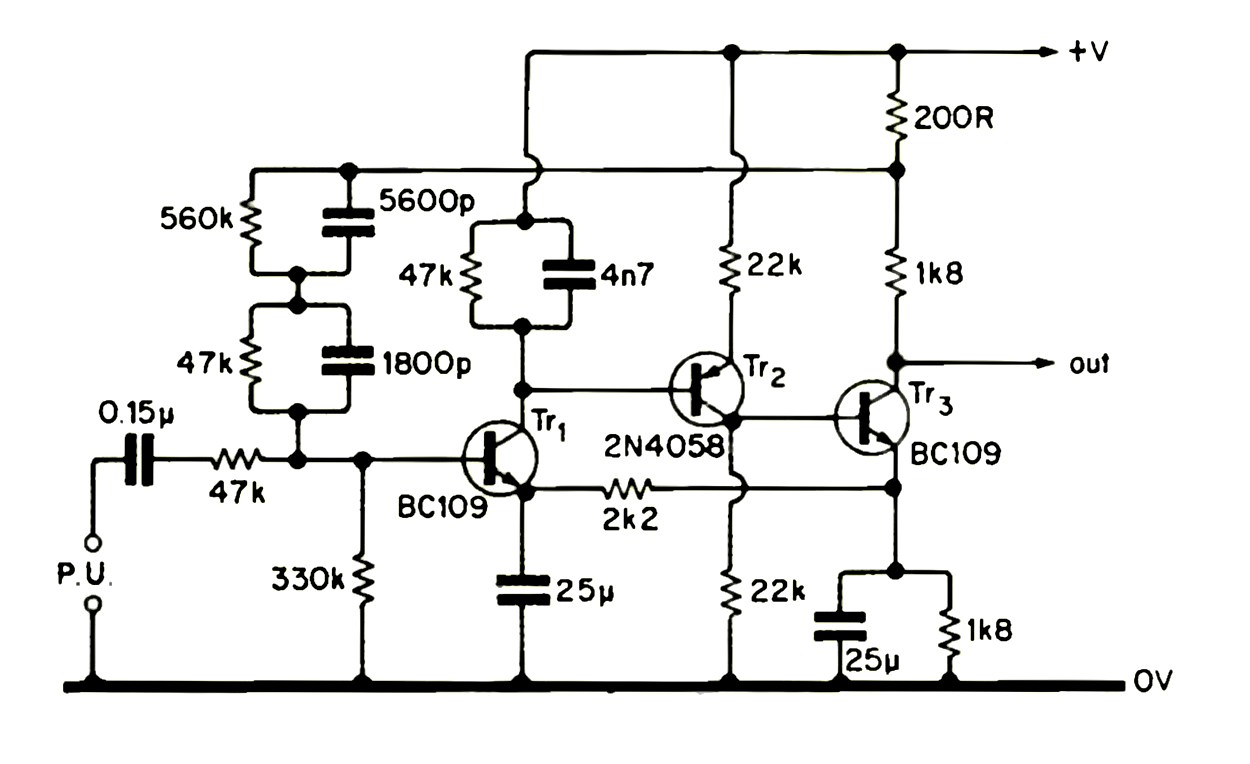
For obscure reasons, the virtual-earth topology of RIAA preamplifier was very popular in the valve and early transistor era. Two designs illustrate this; one from the 1950s and the other from the 1960s.¹
Two practical RIAA feedback preamplifiers (virtual-earth type). The pentode design is due to Livy (1957)² and the second due to Linsley Hood (1969)¹
The significant disadvantage of the virtual-earth amplifier stage is the series resistance (Rin). The thermal-noise generated in this resistance is in series with the signal-source impedance and this sets the lower bound on the noise performance of this stage to such an extent that the non-inverting stage arrangement is always used today (although often without the necessary proviso of the extra pole).
Lipshitz and Baxandall conquer all
Combining the equalisation network around an amplifier complicates the transfer-function of the combined circuit because any real amplifier will not be perfect and will have finite gain and frequency-response. In the valve (tube) era, the limitation was normally gain at low-frequencies being insufficient to provide the full bass-boost required. Livy says of his design, ❝...the gain of the valve [may not be] enough to prevent the bass response from flattening off due to the feedback becoming inoperative....❞ ²
The more modern design¹ suffers the limitation of open-loop gain falling with frequency. In Linsley Hood's circuit, this is due to the 4n7 in parallel with the collector load of Tr1, but it is a feature of all modern op-amps too which include dominant-pole compensation to ensure stability.
The whole issue of equalisation networks (there are different arrangements of Cs and Rs) and their combination with amplifiers of finite gain-bandwidth product is covered in a seminal, tour de force of a paper by Lipshitz from 1979.³
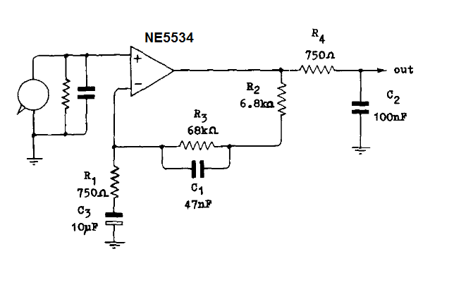
Lipshitz paper should be read with Baxandall's reply in the JAES letters a little later.³ Baxandall suggests a circuit arrangement about which he says, ❝I looked rather carefully into the optimum design of RIAA replay circuits .... and recommended the circuit shown in basic form [below].❞
Baxandall's ❝optimum❞ RIAA preamplifier design
The last word?
Baxandall's "optimum" design represents (roughly) the end-point of practical, hardware RIAA preamplifier design. It sidesteps the noise issue of the virtual-earth arrangement, and it evades the limited attenuation issue of the non-inverting type circuit by moving the 75µs time-constant to a subsequent RC stage (R4, C2). Moving the 75µs time-constant out of the feedback loop also helps prevent any bandwidth issues due to the op-amp complicating the design of the equalisation network.5
In all the forty years since Baxandall's letter³, there have been thousands of elegant variations on this theme, but none appreciably betters Baxandall's design. The more rational variations have included:
Substituing exotic op-amps or discrete, complicated transistor or tube amplifiers instead of an op-amp.
Reducing the value of R1 to reduce its noise contribution.
Using multiple capacitors to improve filter accuracy.
Substitutions involving more exotic op-amps or discrete amplifiers rarely offer tangible improvement, indeed, Self argues convincingly that the humble NE5534 really cannot be beaten in this rôle.8The Appendix covers a discussion concerning the use of multiple capacitors. None of the above can qualify as substantial improvements.
It was the belief that RIAA preamplifier design had "run out of road" which provoked us to developing RIAA equalisation in software in Stereo Lab because, although Baxandall's circuit is excellent, along with any other piece of analogue electronic hardware, it isn't perfect. A couple of examples of practical limitations are given below.
Monte Carlo (or Bust)
Any practical, analogue circuit uses commercial electronic components supplied as having a particular value (6800Ω for example) with a particular tolerance (± 10%, ± 1% etc.).
The performance of Baxandall's circuit may be analysed today in ways unavailable at the time of its conception. Using computer circuit-simulation software, we can plot all the variations due to the tolerance variations of every one of the circuit components. Known as a Monte Carlo analysis, such an audit would have been unthinkable in the days of the pocket calculator — let alone the slide-rule.³
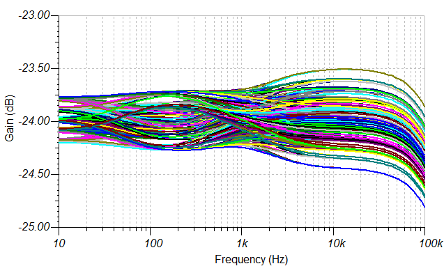
Using simulation software, we can generate a curve for every permutation of every tolerance variation in the circuit and we can display all these curves together in a graphic we call a response skein because it looks like loose-coiled yarn of different colours. This response skein illustrates the performance spread of the circuit; the outer traces illustrating the worst-case variations.
In the analysis plotted here, resistors are taken to have a ±1% tolerance and capacitors a ±2% tolerance. These are the tolerances representative of the components used in high-quality hardware preamplifiers.
The input was mathematically manipulated to the transfer-function (equation A) and is thus RIAA pre-equalised. A perfect result would therefore be a straight-line. Depending on luck of the draw, in terms of the combination of real electronic component values in any hardware example of this circuit, the analysis illustrates that frequency-response may not be guaranteed to be better than about ±0.5dB.
Naturally, in a digital implementation, as in Stereo Lab, there is no need to accept any variation from the exact transfer-function of equation (B).
The 10µF electrolytic capacitor (C3) was left out of this Monte Carlo analysis. The rôle of this capacitor is to provide rumble filtering by rolling-off the response at low-frequencies. A capacitor of some value is required in any real hardware design to keep the offset voltage of the op-amp under control by returning the loop-gain to 0dB at DC. It does double-duty as a rumble-filter here. If this component is included, the response variation is very much worse because electrolytic capacitor values tolerance are rarely better than ±10%.
Component C3 in Baxandall's design is chosen approximately to implement the, so called IEC amendment, which specifies in a further time constant at 7950µS for rumble and warp handling in the IEC version of the replay equaliser standard.6 (10µF × 750Ω = 7500µs)
Whilst this very gradual high-pass technique provides some protection against rumble, warp and arm resonance, it doesn't do a great job. Worse, it affects wanted frequencies in the lowest musical octave.
Some RIAA preamplifier designs implement a multi-pole high-pass filter after the RIAA equalisation stage. A good example of a practical rumble filter (designed by Doug Self)7 is shown here (left). This design not only rejects the subsonic garbage with an ultimate attenuation of 18dB/octave, but - by virtue of a slightly overdamped response - also implements the IEC roll-off being down -3dB at 20Hz. This is clever design. But it cannot escape physics and a filter of this sort introduces very considerable phase-shift near the turnover frequency.
Now, the term phase-shift causes a lot of confusion in audio. The problem is the concept of phase itself which was principally developed for consideration of the relative delay between currents and voltages in single-frequency power circuits. The concept is much less suitable when considering wideband electrical phenomena.
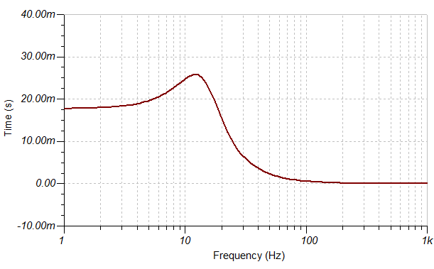
What we need is a measure of how phase changes with respect to frequency. Such a measure exists. It is called group-delay whereby,
Group delay = dφ/dF
That's to say, group delay is defined as the rate of change of phase (dφ) with respect to the rate of change of frequency (dF). So, far better than saying, “a non-distorting circuit has a linear phase response,” better to say that a non-distorting circuit has a “constant group-delay,” because dφ/dF is a constant.
When group delay is not constant, signal components of one frequency arrive before or after signal components of other frequencies and that is the key to understanding the graph of the group delay of Self's rumble circuit which delays frequencies around the cut-off by 20mS with respect to the mid-band frequencies. Given that the speed of sound in air is about 340m/s, a delay of 20mS represents a delay equivalent to nearly seven metres as if the woofer of a loudspeaker was placed 7metres further away than the mid-range unit!
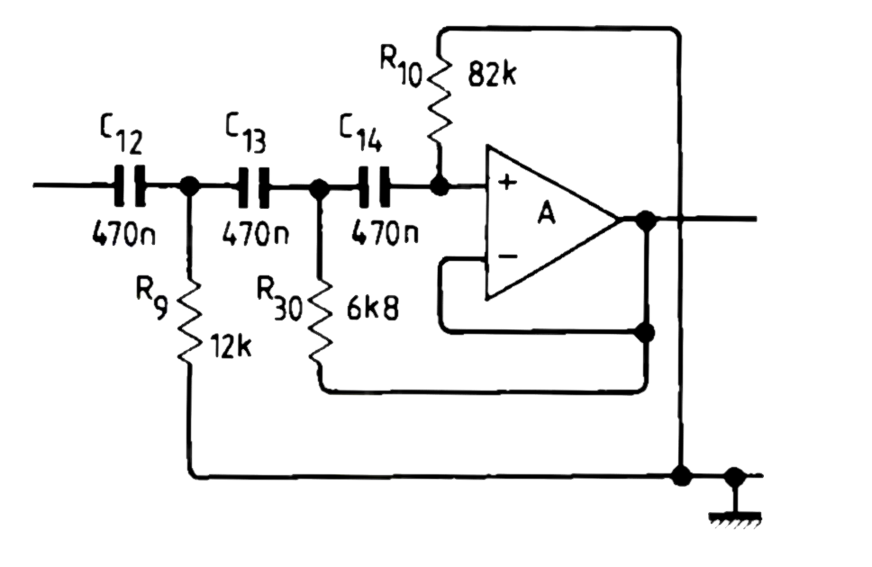
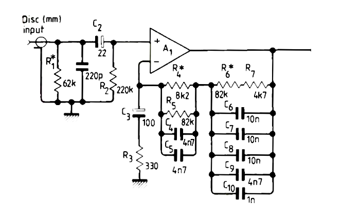
Shown right is a preamplifier design from 1983 which uses multiple capacitors to achieve a larger capacitance from a combination lower-value components. There exists some statistical advange in using multiple components of the same value in filter circuits.7,8
The three 10nF capacitors (C6, C7, C8) in parallel reduce the tolerance from the nominal 2.5% of the manufacturer's tolerance for each individual component, to 1.44% tolerance for the 30nF combination.
This kind of "tolerance improvement strategy" has the following characteristics: it improves the average behaviour by a factor of √(n) where n components of the same value are used. (So 2.5% ⁄ √3 = 1.44%.)
Similarly, the average tolerance of the two 4n7 components (C4, C5) is improved by 1 ⁄ √2.
But, note the term average. The technique does not improve the worst-case behaviour as revealed in the Monte Carlo analysis technique above. If all components have maximum positive or negative deviations from their nominal values then the worst case performance is still determined by the tolerance of the individual capacitances.
In other words, the multiple component technique improves the chances of getting a component with a better tolerance, but it doesn't reduce the performance spread. Equalisation accuracy specifications based on calculation of tolerance improvement by combinations of components are thereby misleading.
Furthermore, Gert Willmann has pointed out9 that the technique only works when the individual component values are not correlated and there are no systematic production-based dependencies. The technique will not work where the distribution of the components is not normal (Gaussian).
A manufacture's tolerance of ±10% may be taken as a reliable indication that "most" supplied components will be within a 10 percent margin either side of annotated value. But what is the distribution of values within the tolerance range?
Normal is the Holy Grail10
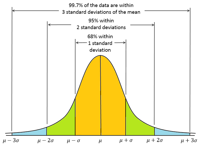
When lots of data are collected concerning all manner of phenomena, they tend to be distributed around a central value in something called a normal (or Gaussian) distribution.
Plotted as a graph (as a probability density function, right), the graph is sometimes called a bell curve — a silly term because the essential feature of the normal distribution is that the slopes on either side of the curve descend, in an ever shallower slope, for ever. Just the way that the sides of a bell don't!
This normal distribution of the individual values in a large-scale data-set is true of: people's heights; errors in measurements; blood pressure; pizza delivery times; and exam marks. It is very often true of a dimension of a manufactured product, like the size or weight of a cookie..... and maybe of resistors and capacitor values.
Standard deviation (σ)
In any normal distribution, the percentage of data values which lie within bands around the mean (annotated µ) is predictable. These bands are called standard deviations (annotated with a lower-case sigmaσ)11. As the graph shows, 68% of all the data values will be distributed within ±1 standard deviations of the mean (µ ± σ). A further 27% will be distributed within ± 2 standard deviations of the mean (µ ± 2σ). For all sorts of practical purposes, 99.7% of the data (which we might like to call "nearly all" or something similar) will be distributed within ± 3 standard deviations of the mean (µ ± 3σ).
To extend the information in the graphic, note that:
Range
Percentage of population
µ ± σ
68.268949%
µ ± 2σ
95.449974%
µ ± 3σ
99.730020%
µ ± 4σ
99.993666%
µ ± 5σ
99.999942%
µ ± 6σ
99.999999%
Is the distrubution of resistor, or capacitor values normal?
The definitive answer to this is frustratingly not known. It's a reasonable assumption to suppose it is. But, even if we assume a normal distribution, we don't know the standard deviation. So we don't know if one in a thousand resistors will be out of range, or one in a million. Manufacturer's data sheets don't seem to specify this at all.
Here is a good and interesting video on this subject (it's a bit long — stick with it).12 The video contains solid, empirical work. It suggests the (1kΩ) resistors in question display a manufactured tolerance distribution which is normal and with a standard-deviation of about 2Ω such that only about 1 value in 400 (the sample size) approached the ±0.6% value. This suggests a process with something like a 5σ distribution, so that only resistor in about 2 million will be on the limit of the tolerance specification. But we can't take it for granted this applies to all components.
Most analogue design engineers know an anecdote (believed to be true) about a study of 10kΩ ±10% resistors. Measured resistance values of a sizeable batch of components (just like that performed by Dave Jones12) revealed that all the values fell within the 9k to 11k range as expected. However, none of the batch fell on the precise value of 10kΩ — or indeed on any value 100Ω either side of the annotated value. Clearly, the ±10% range was from a batch of components from which ±1% had already been selected.
Not only does this mean the distribution of the ±10% values would be non-Gaussian, but the 1% components, obtained by selection wouldn't display a normal distribution either. The trick of using multiple components to improve the probability of better accuracy would not apply for either of these populations.
References and Notes
1. Audio Preamplifier Design (part. 1) Linsley Hood, J. Electronics World and Wireless World June 1990
3. On RIAA Equalization Networks. Lipshitz, S.P Journal of the Audio Engineering Society Vol. 27 No. 6 1979 June. Also see Comments On RIAA Equalization Networks (letters to the editor). Baxandall, P. J. Audio Eng. Soc., Vol. 29, No. 1/2, 1981 Jan./Feb.
4. Disc preamplifier. Brice, R. Electronics and Wireless World June 1985
5. Although Baxandall does say, ❝Modern wide-band low-noise integrated operational amplifiers, such as the Signetics NE5534AN have such excellent performance that there is little need to allow for the effects of finite gain in the analysis, even when quite high accuracy of response is required.❞
6. IEC 60098:1987 Analogue audio disk records and reproducing equipment. Available at: https://webstore.iec.ch/publication/734 . This extra roll-off (the ‘IEC Amendment’) and it was added to IEC 98 in 1976
7. Precision preamplifier. Self, D. Wireless World October 1983
8. Small Signal Audio Design. Self, D. Focal Press; 2nd edition (2014)
9. Private correspondence.
10. Sarah Crossan (Irish author)
11. Standard deviation is defined at the square-root of the variance where the variance is the average of the squared differences from the mean of all the data. So, if the data is: a, b, c, d, and e, The mean (µ) is the sum of a + b + c....+ e divided by five: the variance (σ²) is [(µ - a)² +(µ - b)²....... +(µ - e)²] ÷ 5. And the standard deviation is the square-root of the variance.
14. New factors in phonograph preamplifier design. Holman, T. JAES Vol. 24, No. 4 May 1976.
Holman's article pioneered the idea that phono preamplifiers required a huge overload margin, so that maximum input to an MM phono stage of 270mV pk-pk (95mV RMS) should be engineered. This figure sent a generation of design engineers (including us, see note. 4) down an unnecessary path. Holman's reasoning was to take the figure for maximum recorded velocitiy, assume the cartridge will track at that velocity, and multiply that by the output voltage from the most sensitive moving-magnet cartridge on the market (whilst admitting that the best tracking cartridges have lower sensitivities). In fairness, he does say ❝It should be emphasized that this is a genuinely worst case combination which is not expected to be approached typically in practice.❞, but this misleading figure became, and still is, very influential; see reference 8. We have here a perfect example of the time-warp which surrounds so much information about records.

 Group delay = dφ/dF
 Shown right is a preamplifier design from 1983 which uses multiple capacitors to achieve a larger capacitance from a combination lower-value components. There exists some statistical advange in using multiple components of the same value in filter circuits.7,8
 A manufacture's tolerance of ±10% may be taken as a reliable indication that "most" supplied components will be within a 10 percent margin either side of annotated value. But what is the distribution of values within the tolerance range?